NSGA-II

Non-dominated Sorting Genetic Algorithm II combines Pareto ranking with crowding distance to select a diverse population. Use this page to run and understand a two-objective example. For exact signatures and builder methods, use the separate NSGA-II configuration reference.

All algorithms · Define your own problem · Result API

Run an example

This example uses ZDT1 with 30 real variables, a population of 100, a budget of 10,000 evaluations, the NumPy backend, and seed 42. These are the settings of this tutorial, not a tuned configuration or a claim of superiority over other algorithms. Follow the installation guide first; optimization itself does not require plotting dependencies.

from vamos import optimize
from vamos.algorithms import NSGAIIConfig
from vamos.problems import ZDT1

problem = ZDT1(n_var=30)
config = NSGAIIConfig.default(pop_size=100, n_var=problem.n_var)
result = optimize(
    problem,
    algorithm="nsgaii",
    algorithm_config=config,
    max_evaluations=10_000,
    engine="numpy",
    seed=42,
)

print(result.X.shape)  # (number of returned solutions, 30)
print(result.F.shape)  # (number of returned solutions, 2)
print(result.data["evaluations"])  # 10000 for this uninterrupted run

The complete executable example runs the same configuration and can also generate the illustration. From a checkout with VAMOS installed:

python examples/journeys/nsgaii_zdt1.py

Understand the result

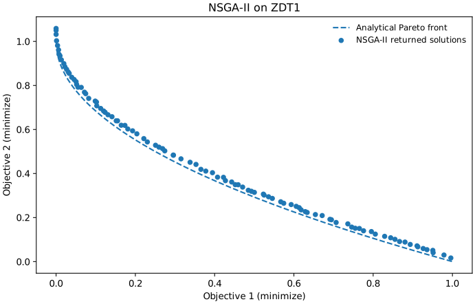
Illustrative run: NumPy, seed 42, population 100, 10,000 evaluations. The points are computed by the linked script, not drawn by hand. The dashed curve is an analytical reference, not another optimization run.

Each row result.X[i] is a decision vector; result.F[i] contains its two objective values. Moving towards the lower-left improves both objectives, but along the trade-off curve an improvement in one objective costs performance in the other. There is no single preferred solution without an additional decision criterion.

For this unconstrained example, result.F contains the non-dominated solutions selected from the final population. Its row count is not guaranteed to equal the population size. The complete final population is available through result.data["population"]. The result API describes the container and its selection helpers.

For ZDT1, the reference curve is f2 = 1 - sqrt(f1) for 0 <= f1 <= 1. The reference does not guide this NSGA-II run. The visible distance to it is residual approximation error: a completed budget does not guarantee convergence. A single seed and one problem do not establish comparative performance.

To generate your own SVG, install the plotting dependency and choose a new output filename:

python -m pip install matplotlib
python examples/journeys/nsgaii_zdt1.py --output nsgaii-zdt1.svg

The script refuses to overwrite an existing file. A short smoke run uses --pop-size 20 --max-evaluations 200; it tests execution, not convergence, and will not reproduce the illustration above.

How selection works

For the generational configuration used here, the algorithm repeatedly performs the following cycle [1]:

1. Select parents, then apply crossover and mutation to create offspring.
2. Evaluate offspring and combine them with the current population.
3. Sort the combined solutions into non-dominated fronts. Prefer lower-rank fronts.
4. Fill the next population with complete fronts; when the final accepted front does not fit, prefer larger crowding distances within that front.

Crowding distance estimates local spacing in objective space using normalized neighbouring objective differences. Boundary solutions receive special treatment to preserve extremes. It is a diversity criterion, not a distance to the true Pareto front. In the tutorial configuration, tournament selection also uses rank and crowding.

This is the algorithmic idea. The encoding, variation operators, constraint handling, result selection and optional archives below are implementation/configuration choices that must be reported separately when comparing runs.

Configure the run

NSGAIIConfig.default(...) is a convenient starting point. Supplying n_var makes its mutation probability depend on the actual problem dimension. To make the tutorial's real-coded variation explicit, use the builder:

from vamos.algorithms import NSGAIIConfig

config = (
    NSGAIIConfig.builder()
    .pop_size(100)
    .crossover("sbx", prob=1.0, eta=20.0)
    .mutation("pm", prob="1/n", eta=20.0)
    .selection("tournament", size=2)
    .build()
)

Pass that config as algorithm_config to optimize() as above. The string "1/n" resolves using the problem's number of variables; for the 30-variable example it is 1/30.

Steady-state NSGA-II

The default configuration is generational: when offspring_size is omitted, the runtime uses pop_size, so a full offspring batch is evaluated before survival. For the classic one-offspring steady-state variant, use the explicit .steady_state() builder switch:

from vamos.algorithms import NSGAIIConfig

steady_state_config = (
    NSGAIIConfig.builder()
    .pop_size(100)
    .steady_state()
    .crossover("sbx", prob=1.0, eta=20.0)
    .mutation("pm", prob="1/n", eta=20.0)
    .selection("tournament", size=2)
    .build()
)

Pass steady_state_config to optimize() as algorithm_config. .steady_state() resolves the configuration to offspring_size=1 and replacement_size=1. VAMOS therefore creates and evaluates one offspring, combines it with the current population, and applies NSGA-II survival back to pop_size after every offspring evaluation. Explicit contradictory values such as .steady_state().offspring_size(20) fail fast rather than silently changing the requested mode.

The initial population still counts towards max_evaluations. With pop_size=100 and max_evaluations=10_000, the first 100 evaluations initialize the population and the remaining 9,900 evaluations are one-offspring steady-state steps. The older explicit .offspring_size(1) form remains supported and reaches the same one-offspring execution path, but .steady_state() is the clearer public spelling. Values 1 < offspring_size < pop_size instead use smaller incremental batches; they are not the classical one-offspring steady-state case.

When comparing generational and steady-state NSGA-II, keep the evaluation budget and seed policy explicit. Changing the replacement schedule changes the search dynamics even when the total number of evaluations is identical.

Choice	What to consider
pop_size	Changes population cardinality and the allocation of a fixed evaluation budget. A larger value is not automatically better.
.steady_state()	Preferred explicit switch for classic one-offspring steady-state NSGA-II; resolves offspring and replacement sizes to 1.
offspring_size	When omitted, the runtime uses population size. 1 remains a compatible one-offspring spelling; intermediate values use smaller incremental batches.
Crossover and mutation	Choose operators compatible with the problem encoding. The SBX/polynomial-mutation example above is real-coded.
max_evaluations	Includes evaluation of the initial population. The budget must be large enough to initialize it.
seed and engine	Record both, together with the environment and resolved configuration.

This table explains decisions rather than duplicating every signature and default. The configuration reference is generated directly from the implementation.

VAMOS capabilities and limits

The default factory has branches for real, binary, integer, permutation and mixed encodings. For a non-real problem, provide its actual encoding to NSGAIIConfig.default(...); using a real-coded configuration is not an encoding conversion. Consult the problem contracts and custom-problem guide, particularly for mixed-variable specifications. This tutorial validates the real-coded ZDT1 path, not every possible operator/problem combination.

With the default feasibility constraint mode, feasible candidates are favoured over infeasible ones; selection then uses objective space among feasible candidates and total violation among infeasible candidates. Constraints use the G <= 0 convention. The present ZDT1 example has no constraints; follow the custom-problem guide for a constrained problem rather than inferring feasibility from an objective scatter plot.

Without an external archive, the default result mode is non_dominated; population returns the final population. Enabling an external archive changes the default source of returned solutions unless population mode is requested explicitly. The archive is not the population: inspect result.data["archive"] and result.data["population"] separately. See stopping and archives before changing either policy.

The 1.x stability policy defines the supported public surface. Reusing a seed is not a promise of bitwise identity across backends or environments. Use saved runs, verification and replay to retain the resolved configuration and environment for a reproducible workflow.

Continue

Replace ZDT1 using your own objective function, or organize multiple algorithms, problems and seeds as a durable study. The algorithm index links to the other built-in configurations without making an unsupported performance ranking.

References

[1] Deb, K., Pratap, A., Agarwal, S., and Meyarivan, T. (2002). A fast and elitist multiobjective genetic algorithm: NSGA-II. IEEE Transactions on Evolutionary Computation, 6(2), 182–197.

For example/figure provenance and maintenance, see algorithm documentation.