MOEA/D

Multiobjective Evolutionary Algorithm based on Decomposition assigns a scalar subproblem to each weight vector and shares solutions between neighbouring subproblems [1]. This tutorial runs an unconstrained, real-coded example using the stable public API in VAMOS 1.0.0.

All algorithms · Configuration reference · Installation

Run an example

Use ZDT1 with 30 variables, 100 subproblems, 10,000 evaluations, NumPy, and seed 42. The initial population counts towards the budget. These settings illustrate the workflow; they are not tuned or evidence of comparative performance.

from vamos import optimize
from vamos.algorithms import MOEADConfig
from vamos.problems import ZDT1

problem = ZDT1(n_var=30)
config = MOEADConfig.default(
    pop_size=100, n_var=problem.n_var, n_obj=problem.n_obj
)
result = optimize(
    problem,
    algorithm="moead",
    algorithm_config=config,
    max_evaluations=10_000,
    engine="numpy",
    seed=42,
)
print(result.X.shape)  # (number of returned solutions, 30)
print(result.F.shape)  # (number of returned solutions, 2)
print(result.data["evaluations"])  # 10000

The executable example uses precisely these settings. From a checkout with VAMOS installed:

python examples/journeys/moead_zdt1.py

Understand the result

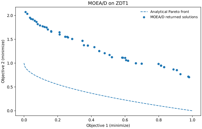
Actual run: VAMOS 1.0.0, NumPy, seed 42, 100 subproblems, 10,000 evaluations. The dashed curve is analytical, not another run.

Each row of X is a decision vector and the corresponding row of F gives its objectives. The default result mode selects non-dominated solutions from the final population, so the number returned need not equal 100. Inspect result.data["population"] for the whole final population. The visible gap to the dashed curve shows that this default configuration has not converged at the chosen budget: a non-dominated result can still be far from the true front. The figure intentionally shows that residual error instead of treating budget completion as a quality guarantee.

For ZDT1 the analytical front is f2 = 1 - sqrt(f1), with 0 <= f1 <= 1. It is shown to help assess the result; it is not supplied to the optimizer. The weights used by MOEA/D are directions in objective space, not points on that front, and are not preferred solutions specified by a user.

To regenerate the illustration at a new path:

python -m pip install matplotlib
python examples/journeys/moead_zdt1.py --output moead-zdt1.svg

Existing files are refused. For a fast execution check, use --pop-size 20 --max-evaluations 203; this deliberately short run does not reproduce the illustration's approximation quality.

What the configuration means

The default real-coded configuration uses differential evolution (cr=1.0, f=0.5), polynomial mutation (eta=20, probability 1/n_var), PBI aggregation (theta=5), neighbour size 20, neighbourhood selection probability 0.9 and replacement limit 2. These are VAMOS configuration choices, not a claim that every MOEA/D variant uses them.

Decision	Consequence
Population and weights	One incumbent is associated with each weight vector; use matching cardinalities.
Neighbour size	Controls how many nearby weight vectors participate in local cooperation.
delta	Controls how often mating draws from the neighbourhood rather than the whole population.
Aggregation	PBI, Tchebycheff and weighted sum define different scalar subproblems; objective scales and front geometry affect the choice.
Replacement limit	Bounds how many incumbents one new solution can replace.
batch_size	The tutorial uses one generated candidate per step; changing batching changes search dynamics.

For two objectives, MOEADConfig.default(pop_size=100, n_obj=2, ...) requests 99 divisions and therefore 100 uniformly spaced weights. For m objectives and a simplex lattice with p divisions, the count is comb(p + m - 1, m - 1). For example, three objectives and 12 divisions give 91, not 100. Explicit files must also contain exactly one vector per population member. Incompatible cardinalities raise an error; budget reduction is not a way to repair a mismatched configuration.

The n_obj argument matters: the default factory otherwise assumes three objectives. Supply the real problem dimension and objective count as above. Its default operators are real-coded; for discrete problems, choose compatible operators through the builder or the encoding-aware optimization setup. See the capability matrix.

Constraints, archives and reproducibility

This example is unconstrained. MOEA/D supports feasibility-based comparison with the G <= 0 convention; the constraint reference explains how to supply residuals. A scatter plot of objectives alone does not establish feasibility.

An optional external archive stores non-dominated results separately from the working population. Choose result_mode="population" explicitly when the final population is the required output; otherwise an enabled external archive becomes the result source. The MOEADConfig reference documents result-archive configuration. The stopping and archive hooks maintain a separate objective-space observation archive. Preserve the resolved configuration, effective backend and seed with the run lifecycle.

References

[1] Zhang, Q., and Li, H. (2007). MOEA/D: A Multiobjective Evolutionary Algorithm Based on Decomposition. IEEE Transactions on Evolutionary Computation, 11(6), 712–731.