IBEA

Indicator-based selection turns pairwise objective comparisons into fitness [1]. Here the additive epsilon indicator drives search; the indicator chosen for selection need not be the metric used to report final quality.

Goal: run the stable public API in VAMOS 1.0.1, interpret its returned population, and identify which settings control this mechanism.

Capability matrix · Exact configuration reference · Setup and recorded evidence

Run the example

Prerequisite: complete T01 and the coverage setup. The protocol uses ZDT1, 10 real variables, 2 objectives, population 40; 400 evaluations; NumPy; seed 42. Initial evaluations count towards the budget. Settings are illustrative, not tuned.

python ibea.py
python ibea.py --output ibea-local.svg

The second command reruns the same protocol and requires Matplotlib. Use a new filename.

Download the complete script.

Complete runnable script

"""Verified VAMOS 1.0.1 lesson: ibea. See coverage-setup for dependencies."""


def execute_example(problem, algorithm, config, budget, seed=42, engine="numpy"):
    import numpy as np

    from vamos import OptimizationResult, optimize

    result = optimize(problem, algorithm=algorithm, algorithm_config=config, max_evaluations=budget, seed=seed, engine=engine)
    G = result.data.get("G")
    if getattr(problem, "n_constraints", 0) and G is None:
        raise ValueError("Declared constraints are missing from the returned result.")
    feasible_rows = np.arange(len(result.F)) if G is None else np.flatnonzero(np.all(G <= 0, axis=1))
    if len(feasible_rows):
        feasible = OptimizationResult({"X": result.X[feasible_rows], "F": result.F[feasible_rows]})
        front, local = feasible.front(return_indices=True)
        front_rows = feasible_rows[local]
    else:
        front, front_rows = np.empty((0, problem.n_obj)), np.empty(0, dtype=int)
    print(f"Algorithm: {algorithm}; encoding: {problem.encoding}; backend: {engine}; seed: {seed}")
    print(f"Returned X: {result.X.shape}; F: {result.F.shape}; result mode: population")
    print(f"Feasible rows: {len(feasible_rows)}/{len(result.F)}; feasible non-dominated rows: {len(front)}")
    print(f"Evaluations: {result.data['evaluations']}")
    return {
        "problem": problem,
        "algorithm": algorithm,
        "config": config,
        "result": result,
        "feasible_rows": feasible_rows,
        "front": front,
        "front_rows": front_rows,
    }


def run_ibea(budget=400):
    from vamos.algorithms import IBEAConfig
    from vamos.problems import ZDT1

    problem = ZDT1(n_var=10)
    config = (
        IBEAConfig.builder()
        .pop_size(40)
        .crossover("sbx", prob=1.0, eta=20.0)
        .mutation("pm", prob=1.0 / problem.n_var, eta=20.0)
        .selection("tournament")
        .indicator("eps")
        .kappa(1.0)
        .result_mode("population")
        .build()
    )
    return execute_example(problem, "ibea", config, budget)


def plot_example(data, output):
    from pathlib import Path

    import matplotlib

    matplotlib.use("Agg")
    import matplotlib.pyplot as plt
    import numpy as np

    output = Path(output)
    if output.exists():
        raise FileExistsError(f"Choose a new figure filename: {output}")
    if output.suffix.lower() != ".svg":
        raise ValueError("Use an .svg output filename.")
    f = data["result"].F
    with plt.rc_context({"svg.hashsalt": "vamos-coverage", "svg.fonttype": "none"}):
        fig = plt.figure(figsize=(7, 4.5), layout="constrained")
        if f.shape[1] == 3:
            ax = fig.add_subplot(projection="3d")
            ax.scatter(*f.T, c="#007f7a", s=22)
            ax.set(xlabel="f1", ylabel="f2", zlabel="f3")
            ax.set_box_aspect((1, 1, 0.85), zoom=0.85)
        else:
            ax = fig.add_subplot()
            ax.scatter(*f.T, c="#b6bec8", s=25, label="Returned population")
            if len(data["front"]):
                ax.scatter(*data["front"].T, c="#007f7a", s=30, label="Feasible non-dominated rows")
            labels = {
                "WeldedBeamDesignProblem": ("Cost (minimize)", "Deflection proxy (minimize)"),
                "FeatureSelectionProblem": ("Validation error (minimize)", "Feature count (minimize)"),
                "HyperparameterTuningProblem": ("Validation error (minimize)", "Complexity proxy (minimize)"),
            }
            xlabel, ylabel = labels.get(type(data["problem"]).__name__, ("f1 (minimize)", "f2 (minimize)"))
            ax.set(xlabel=xlabel, ylabel=ylabel)
            ax.legend()
        if data["problem"].__class__.__name__ in {"ZDT1", "ZDT1Problem"}:
            x = np.linspace(0, 1, 101)
            ax.plot(x, 1 - np.sqrt(x), "--", c="#7c8795", label="Analytical front")
            ax.legend()
        ax.set_title(f"{data['algorithm'].upper()} · {data['result'].data['evaluations']} evaluations · seed 42")
        fig.savefig(output, metadata={"Date": None}, bbox_inches="tight", pad_inches=0.25)
        plt.close(fig)
    output.write_text("\n".join(line.rstrip() for line in output.read_text(encoding="utf-8").splitlines()) + "\n", encoding="utf-8")


def lesson_cli(function, default_budget=400):
    import argparse

    parser = argparse.ArgumentParser(description="Run a bounded VAMOS example and optionally plot its actual result.")
    parser.add_argument("--budget", type=int, default=default_budget)
    parser.add_argument("--output", help="New SVG filename; requires Matplotlib")
    args = parser.parse_args()
    data = function(budget=args.budget)
    if args.output:
        plot_example(data, args.output)


if __name__ == "__main__":
    lesson_cli(run_ibea, default_budget=400)

Recorded output

Algorithm: ibea; encoding: real; backend: numpy; seed: 42
Returned X: (40, 10); F: (40, 2); result mode: population
Feasible rows: 40/40; feasible non-dominated rows: 15
Evaluations: 400

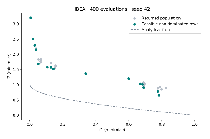
Measured with VAMOS 1.0.1; the observations and provenance retain the inputs and results.

Understand the configuration

Setting	Meaning in this example
indicator("eps")	Uses VAMOS’s epsilon-based fitness path.
kappa(1.0)	Controls scaling in the indicator-to-fitness transformation; it is not an evaluation budget or tolerance.
SBX + polynomial mutation	Real-coded variation with mutation probability 1/10.
Tournament selection	Selects parents using the computed fitness.

Interpret the result and its limits

Each X row aligns with the same F row. This lesson explicitly requests population mode, then computes the feasible non-dominated subset separately. All objectives are minimized. A non-dominated row is only non-dominated among the available rows; it need not be Pareto optimal. The retained observations contain the actual arrays and configuration.

Objective units and the indicator’s scaling affect fitness. Do not infer scale invariance or superior quality from the indicator name. The figure reports objectives in their original units; it does not show a hypervolume-optimized run.

This run has no constraints. Before using a constrained or discrete problem, check the capability matrix and constraint convention. Preserve complete runs through the canonical lifecycle; the teaching JSON is not a replay bundle.

Try one controlled change

Change only kappa to 0.5, preserve the seed and budget, and inspect the result. For a conclusion, repeat the experiment and use a common externally defined measurement protocol.

Next: use T06 to turn this example into a reproducible comparison.

References

[1] Zitzler, E., and Künzli, S. (2004). Indicator-Based Selection in Multiobjective Search. Parallel Problem Solving from Nature — PPSN VIII.