T02. Solve your own constrained problem

Goal

Translate a small model into decisions, objectives, bounds, and a constraint; test the evaluator before searching; then extract feasible trade-offs while preserving their original row indices.

Before you start

Item	This lesson
Prerequisites	T01; Python functions and array rows.
Tested package	VAMOS 1.0.1, Python 3.12; setup and exact tested dependencies.
Dependencies	Core VAMOS and its NumPy dependency; the download is self-contained.
Interface status	Stable make_problem, optimize, OptimizationResult, and front.
Run	NSGA-II, population 40, 400 evaluations, seed 42, NumPy.

Define and check the model

This is the teaching surrogate from Solve your own problem, not a validated physical process. Both objective scores are minimized.

Concept	Definition
Decisions	Temperature set point T in [60, 100]; residence time t in [2, 10].
Energy score	((T - 60) / 40)**2 + 0.25*t/10.
Conversion-shortfall score	(100 - T)/40 + 2/t.
Requirement	T*t >= 450, written as g = 450 - T*t <= 0.

Check three designs by hand: [60, 2] is infeasible (g = 330), [75, 6] lies on the boundary (g = 0), and [90, 8] is feasible (g = -270). The middle design's objective scores are approximately 0.290625 and 0.958333. These probes test the meaning and sign of the model before the optimizer spends its budget.

Complete code

Download t02-constrained-problem.py and run it independently; it does not import T01 or require a repository clone.

python t02-constrained-problem.py

"""T02: generated from examples/tutorials/fundamentals.py; VAMOS 1.0.1, core dependencies only."""


def process_objectives(x):
    temperature, residence_time = x
    energy = ((temperature - 60.0) / 40.0) ** 2 + 0.25 * residence_time / 10.0
    shortfall = (100.0 - temperature) / 40.0 + 2.0 / residence_time
    return [energy, shortfall]


def process_constraints(x):
    temperature, residence_time = x
    return [450.0 - temperature * residence_time]


def solve_process(max_evaluations=400):
    import numpy as np

    from vamos import OptimizationResult, make_problem, optimize

    problem = make_problem(
        process_objectives,
        n_var=2,
        n_obj=2,
        bounds=[(60.0, 100.0), (2.0, 10.0)],
        encoding="real",
        constraints=process_constraints,
        n_constraints=1,
        name="process_design_surrogate",
    )
    result = optimize(
        problem,
        algorithm="nsgaii",
        pop_size=40,
        max_evaluations=max_evaluations,
        engine="numpy",
        seed=42,
    )
    # Recheck the original requirement, then keep all arrays aligned.
    G = np.array([process_constraints(x) for x in result.X])
    feasible_rows = np.flatnonzero(np.all(G <= 0.0, axis=1))
    if len(feasible_rows) == 0:
        raise ValueError("No feasible candidates: revisit the model or budget.")
    feasible = OptimizationResult(
        {
            "X": result.X[feasible_rows],
            "F": result.F[feasible_rows],
            "G": G[feasible_rows],
        }
    )
    front_F, local_indices = feasible.front(return_indices=True)
    return {
        "result": result,
        "G": G,
        "feasible_rows": feasible_rows,
        "feasible": feasible,
        "front_F": front_F,
        "front_indices": feasible_rows[local_indices],
    }


def run_t02(max_evaluations=400):
    probes = ([60.0, 2.0], [75.0, 6.0], [90.0, 8.0])
    for x in probes:
        f = process_objectives(x)
        g = process_constraints(x)[0]
        print(f"Check {x}: F=({f[0]:.6f}, {f[1]:.6f}), g={g:.1f}")
    data = solve_process(max_evaluations)
    result = data["result"]
    print(f"Feasible returned rows: {len(data['feasible_rows'])}/{len(result.F)}")
    print(f"Feasible non-dominated rows: {len(data['front_F'])}")
    print(f"Evaluations: {result.data['evaluations']}")
    return data


if __name__ == "__main__":
    run_t02()

Observed result

Actual output from the recorded wheel environment:

Check [60.0, 2.0]: F=(0.050000, 2.000000), g=330.0
Check [75.0, 6.0]: F=(0.290625, 0.958333), g=0.0
Check [90.0, 8.0]: F=(0.762500, 0.500000), g=-270.0
Feasible returned rows: 40/40
Feasible non-dominated rows: 40
Evaluations: 400

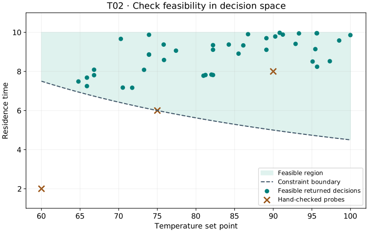
The teal markers are optimized decisions from this run. The brown crosses are the three hand-picked probes, not additional optimization results. The shaded region and dashed boundary come from the stated constraint equation.

Interpret the result

All 40 returned rows happen to be feasible and non-dominated in this execution. That outcome is not a guarantee for a different model, seed, or budget. The code re-evaluates the original requirement and filters infeasible rows before Pareto analysis. If none are feasible, it stops with a clear error.

OptimizationResult here wraps an explicitly filtered in-memory view. It does not launch another search or create a persisted run. The feasible_rows array maps that view back to the original result; applying local_indices to it produces front_indices in the original row numbering. Thus the selected X, F, and G rows still describe the same candidates.

result.front() on its own only Pareto-filters objectives. Neither non-dominance nor a hypervolume score proves that a constraint is satisfied. For numerical equality constraints, define a scientific tolerance deliberately; this example uses the exact inequality g <= 0.

Try one change

Change 450.0 to 600.0 inside process_constraints, then run the script. First predict the new signs for the three probes: 480, 150, and -120. Check those printed values before interpreting any optimized decisions.

The feasible region has changed, so this is a different problem. Do not interpret its objective scores as an algorithm improvement over the original problem. A short run can now return fewer feasible candidates or none.

Next step

Continue with T03. From a Pareto set to a decision. Use the full modeling guide for vectorization, other encodings, simulator boundaries, and common mistakes, or the constraint reference for exact conventions.